Predictions for a new data

Again very similar to PLS — just use method predict() and provide at least matrix or data frame with predictors (which should contain the same number of variables/columns). For test set validation you can also provide class reference information similar to what you have used for calibration of PLS-DA models.

In case of multiple class model, the reference values should be provided as a factor or vector with class names as text values. Here is an example.

res = predict(m.all, Xv, cv.all)
summary(res)

## 
## PLS-DA results (class plsdares) summary:
## Number of selected components: 1
## 
## Class #1 (setosa):
##        X expvar X cumexpvar Y expvar Y cumexpvar TP FP TN FN Spec. Sens. Accuracy
## Comp 1   92.924      92.924   42.703      42.703 25  1 49  0  0.98     1    0.987
## Comp 2    4.560      97.484   11.216      53.920 25  0 50  0  1.00     1    1.000
## Comp 3    1.790      99.274    1.717      55.637 25  0 50  0  1.00     1    1.000
## 
## 
## Class #2 (versicolor):
##        X expvar X cumexpvar Y expvar Y cumexpvar TP FP TN FN Spec. Sens. Accuracy
## Comp 1   92.924      92.924   42.703      42.703  0  0 50 25  1.00   0.0    0.667
## Comp 2    4.560      97.484   11.216      53.920 10  4 46 15  0.92   0.4    0.747
## Comp 3    1.790      99.274    1.717      55.637 10  6 44 15  0.88   0.4    0.720
## 
## 
## Class #3 (virginica):
##        X expvar X cumexpvar Y expvar Y cumexpvar TP FP TN FN Spec. Sens. Accuracy
## Comp 1   92.924      92.924   42.703      42.703 25  4 46  0  0.92  1.00    0.947
## Comp 2    4.560      97.484   11.216      53.920 25  4 46  0  0.92  1.00    0.947
## Comp 3    1.790      99.274    1.717      55.637 24  4 46  1  0.92  0.96    0.933

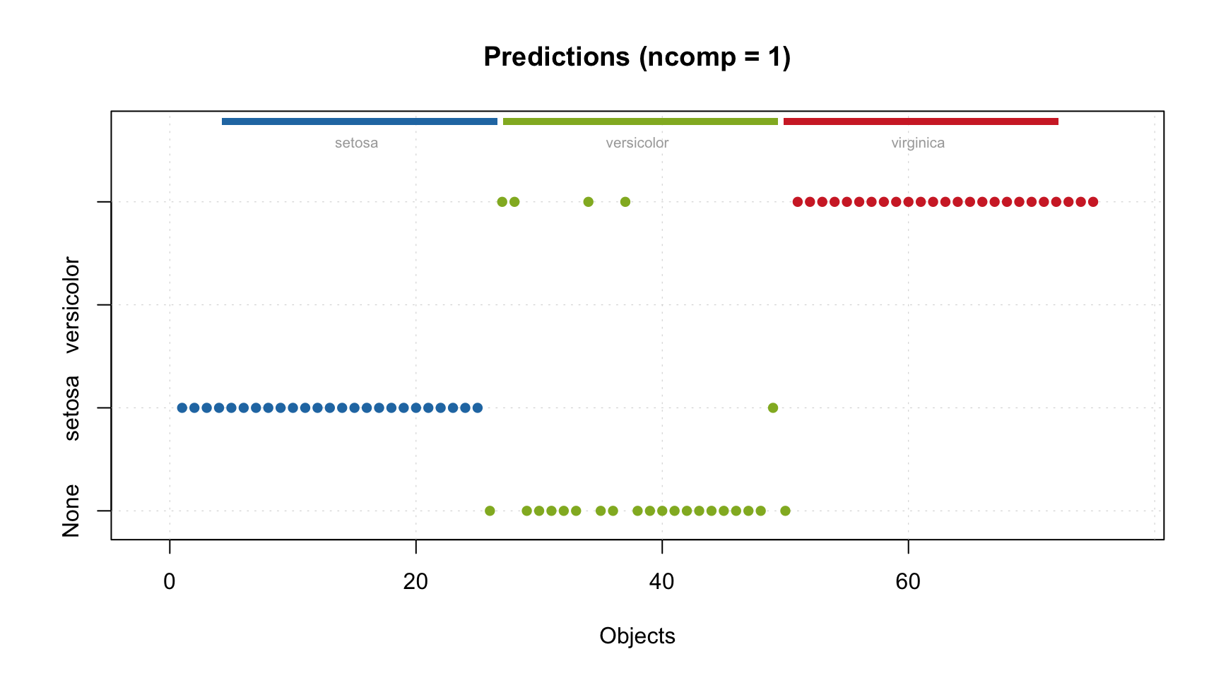
And the corresponding plot with predictions.

par(mfrow = c(1, 1))
plotPredictions(res)

If vector with reference class values contains names of classes model knows nothing about, they will simply be considered as members of non of the known clases (“None”).

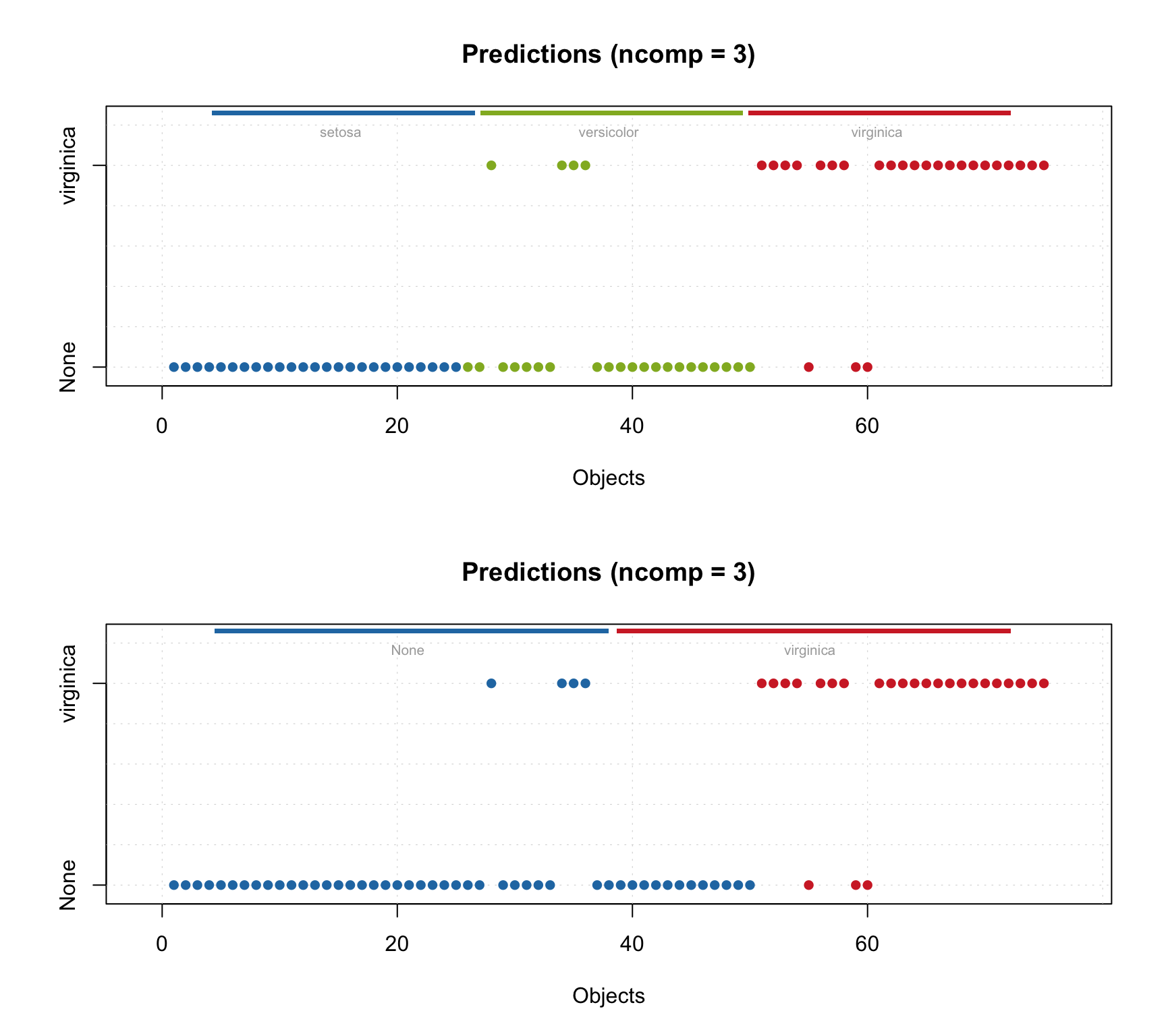
In case of one-class model, the reference values can be either factor/vector with names or logical values, like the ones used for calibration of the model. Here is an example for each of the cases.

res21 = predict(m.vir, Xv, cv.all)
summary(res21)

## 
## PLS-DA results (class plsdares) summary:
## Number of selected components: 3
## 
## Class #1 (virginica):
##        X expvar X cumexpvar Y expvar Y cumexpvar TP FP TN FN Spec. Sens. Accuracy
## Comp 1   93.107      93.107   54.394      54.394 25  4 46  0  0.92  1.00    0.947
## Comp 2    1.588      94.695    6.039      60.433 24  4 46  1  0.92  0.96    0.933
## Comp 3    2.641      97.336   -0.149      60.284 22  4 46  3  0.92  0.88    0.907

res22 = predict(m.vir, Xv, cv.vir)
summary(res22)

## 
## PLS-DA results (class plsdares) summary:
## Number of selected components: 3
## 
## Class #1 (virginica):
##        X expvar X cumexpvar Y expvar Y cumexpvar TP FP TN FN Spec. Sens. Accuracy
## Comp 1   93.107      93.107   54.394      54.394 25  4 46  0  0.92  1.00    0.947
## Comp 2    1.588      94.695    6.039      60.433 24  4 46  1  0.92  0.96    0.933
## Comp 3    2.641      97.336   -0.149      60.284 22  4 46  3  0.92  0.88    0.907

As you can see, statistically results are identical. However, predictions plot will look a bit different for these two cases, as you can see below.

par(mfrow = c(2, 1))
plotPredictions(res21)
plotPredictions(res22)

And because predict() returns an object with results you can also use most of the plots available for PLS regression results. In the last example below you will find plots for X-distance and Y-variance.

par(mfrow = c(1, 2))
plotXResiduals(res21)
plotYVariance(res22)