Regression coefficients
First of all let us re-create the PLS model for prediction of Shoesize from People data we used at the beginning of this chapter:
library(mdatools)
data(people)

idx = seq(4, 32, 4)
Xc = people[-idx, -4]
yc = people[-idx, 4, drop = FALSE]
Xt = people[idx, -4]
yt = people[idx, 4, drop = FALSE]
But this time I will create the model using full cross-validation:
The values for regression coefficients are available in m$coeffs$values, it is an array with dimension nVariables x nComponents x nPredictors. The reason to use the object instead of just an array is mainly for being able to get and plot regression coefficients for different methods. Besides that, it is possible to calculate confidence intervals and other statistics for the coefficients using Jack-Knife method (will be shown later), which produces extra entities.
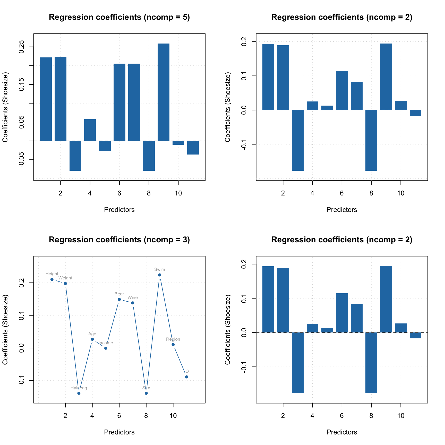
The regression coefficients can be shown as plot using either function plotRegcoeffs() for the PLS model object or function plot() for the object with regression coefficients. You need to specify for which predictor (if you have more than one y-variable) and which number of components you want to see the coefficients for. By default it shows values for the optimal number of components and first y-variable as it is shown on example below.
par(mfrow = c(2, 2))
plotRegcoeffs(m)
plotRegcoeffs(m, ncomp = 2)
plot(m$coeffs, ncomp = 3, type = "b", show.labels = TRUE)
plot(m$coeffs, ncomp = 2)
The model keeps regression coefficients, calculated for centered and standardized data, without intercept, etc. Here are the values for three PLS components.
##       Height       Weight     Hairleng          Age       Income         Beer         Wine          Sex         Swim
##  0.210411676  0.197646483 -0.138824482  0.026613035 -0.000590693  0.148917913  0.138138095 -0.138824482  0.223962000
##       Region           IQ
##  0.010392542 -0.088658626
You can see a summary for the regression coefficients object by calling function summary() for the object m$coeffs like it is shown below. By default it shows only estimated regression coefficients for the selected y-variable and number of components.
However, if you use cross-validation, Jack-Knifing method will be used to compute some statistics, including standard error, p-value (for test if the coefficient is equal to zero in population) and confidence interval. All statistics in this case will be shown automatically with summary() as you can see below.
##
## Regression coefficients for Shoesize (ncomp = 1)
## ------------------------------------------------
##                Coeffs  Std. err. t-value p-value        2.5%       97.5%
## Height    0.176077659 0.01594024   11.03   0.000  0.14310275  0.20905257
## Weight    0.175803980 0.01598815   10.98   0.000  0.14272997  0.20887799
## Hairleng -0.164627444 0.01638528  -10.04   0.000 -0.19852297 -0.13073192
## Age       0.046606027 0.03718827    1.25   0.225 -0.03032377  0.12353583
## Income    0.059998121 0.04047132    1.47   0.155 -0.02372318  0.14371942
## Beer      0.133136867 0.01116749   11.89   0.000  0.11003515  0.15623859
## Wine      0.002751573 0.03542518    0.08   0.936 -0.07053100  0.07603415
## Sex      -0.164627444 0.01638528  -10.04   0.000 -0.19852297 -0.13073192
## Swim      0.173739533 0.01516461   11.44   0.000  0.14236915  0.20510992
## Region   -0.031357608 0.03590576   -0.87   0.395 -0.10563433  0.04291911
## IQ       -0.003353428 0.03841171   -0.08   0.934 -0.08281410  0.07610725
##
## Degrees of freedom (Jack-Knifing): 23
You can also get the corrected coefficients, which can be applied directly to the raw data (without centering and standardization), by using method getRegcoeffs():
##               Estimated
## Intercept  1.251537e+01
## Height     8.105287e-02
## Weight     5.110732e-02
## Hairleng  -5.375404e-01
## Age        1.147785e-02
## Income    -2.580586e-07
## Beer       6.521476e-03
## Wine       1.253340e-02
## Sex       -5.375404e-01
## Swim       1.164947e-01
## Region     4.024083e-02
## IQ        -2.742712e-02
## attr(,"name")
## [1] "Regression coefficients for  Shoesize"