Element wise transformations
Function prep.transform() allows you to apply element wise transformation — when the same transformation function is being applied to each element (each value) of the data matrix. This can be used, for example, in case of regression, when it is necessary to apply transformations which remove a non-linear relationship between predictors and responses.
Often such transformation is either a logarithmic or a power. We can of course just apply a built-in R function e.g. log() or sqrt(), however in this case all additional attributes will be dropped in the preprocessed data. In order to tackle this and, also, to give a possibility for combining different preprocessing methods together, you can use a function prep.transform() for this purpose.
The syntax of the function is following: prep.transform(data, fun, ...), where data is a matrix with the original data values, you want to preprocess (transform), fun is a reference to transformation function and ... are optional additional arguments for the function. You can provide either one of the R functions, which are element wise (meaning the function is being applied to each element of a matrix), such as log, exp, sqrt, etc. or define your own function.
Here is an example:
# create a matrix with 3 variables (skewed random values)
X <- cbind(
   exp(rnorm(100, 5, 1)),
   exp(rnorm(100, 5, 1)) + 100 ,
   exp(rnorm(100, 5, 1)) + 200
)

# apply log transformation using built in "log" function
Y1 <- prep.transform(X, log)

# apply power transformation using manual function with additional argument
Y2 <- prep.transform(X, function(x, p) x^p, p = 0.2)

# show boxplots for the original and the transformed data
par(mfrow = c(1,3))
boxplot(X, main = "Original values")
boxplot(Y1, main = "Preprocessed (log)")
boxplot(Y2, main = "Preprocessed (power)")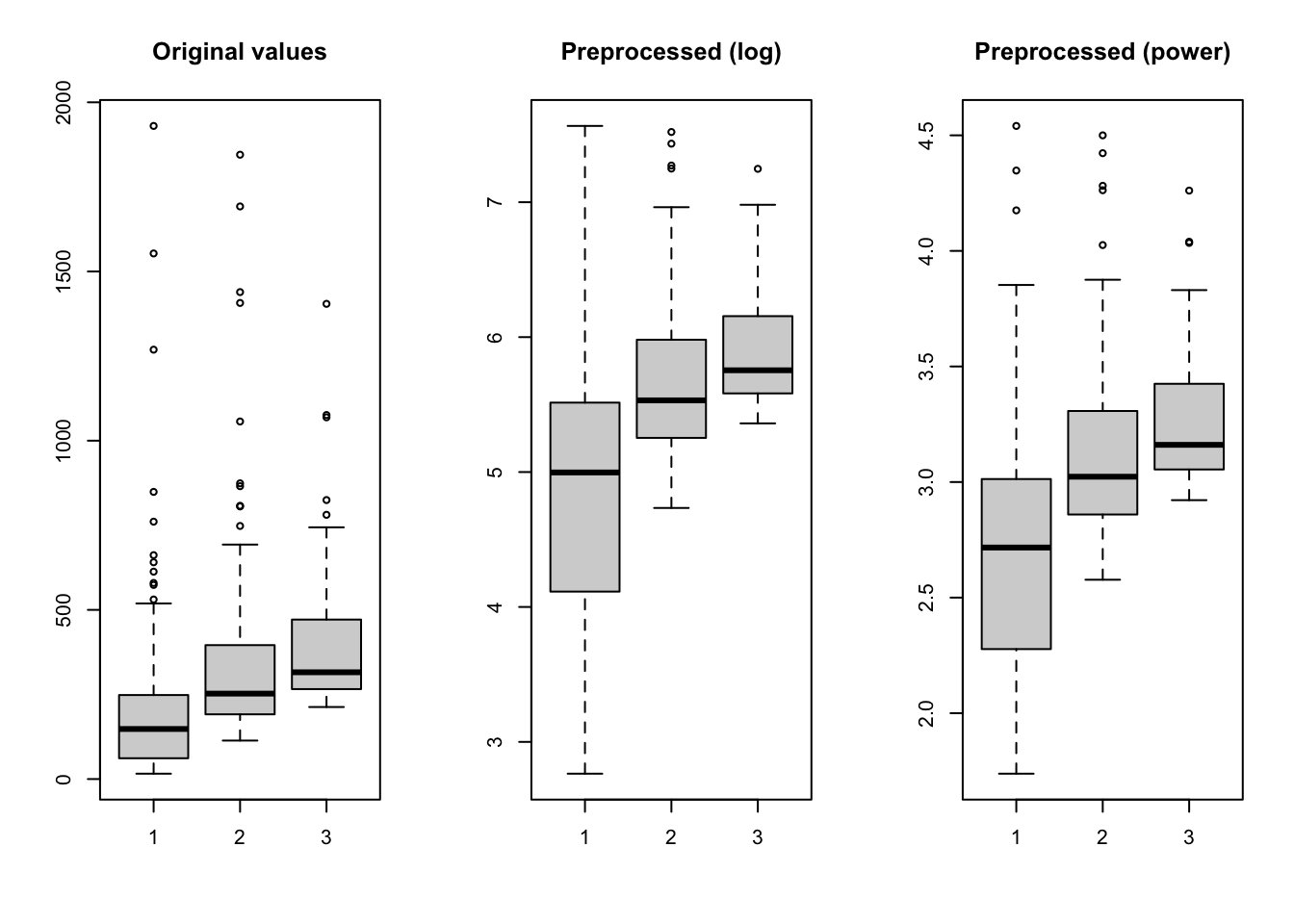
As already mentioned, the prep.transform() preserves all additional attributes, e.g. names and values for axes, excluded columns or rows, etc. Here is another example demonstrating this:
# generate two curves using sin() and cos() and add some attributes
t <- (-31:31)/10
X <- rbind(sin(t), cos(t))
rownames(X) <- c("s1", "s2")

# we make x-axis values as time, which span a range from 0 to 620 seconds
attr(X, "xaxis.name") <- "Time, s"
attr(X, "xaxis.values") <- (t * 10 + 31) * 10
attr(X, "name") <- "Time series"

# transform the dataset using squared transformation
Y <- prep.transform(X, function(x) x^2)

# show plots for the original and the transformed data
par(mfrow = c(2, 1))
mdaplotg(X, type = "l")
mdaplotg(Y, type = "l")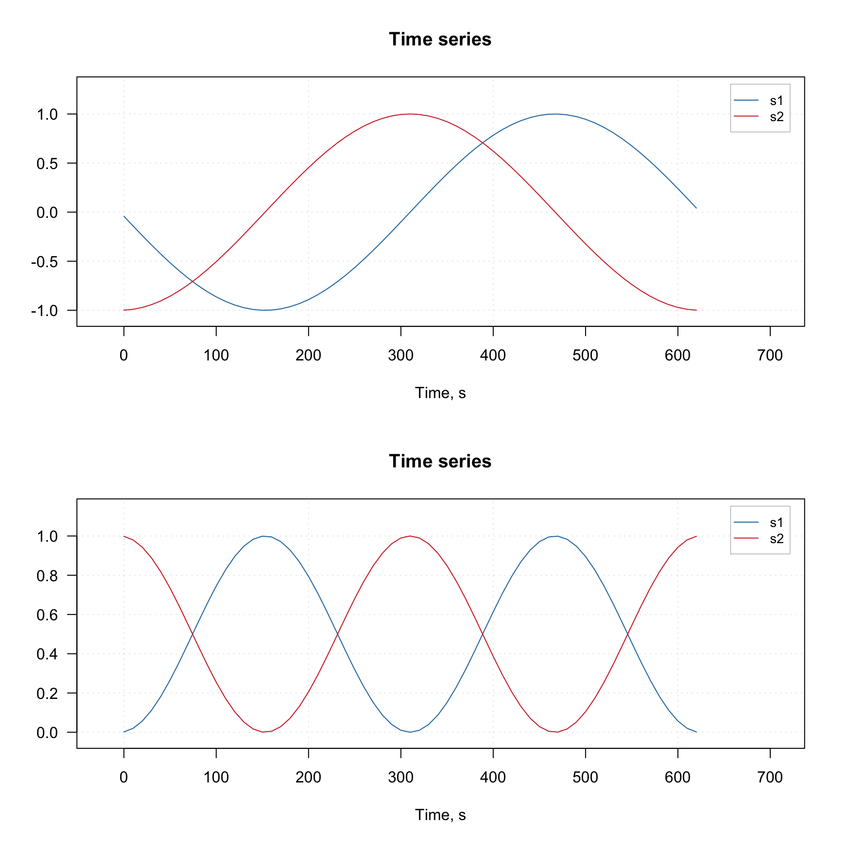
Notice, that the x-axis values for the original and the transformed data (which we defined using corresponding attribute) are the same.